Personalizing Diffusion Models

Evaluation Metrics — How Do I Measure Success?

Before comparing methods, it is important to understand what is being measured. Personalization quality isn't a single number — it has multiple dimensions. A generated image of "your dog on the beach" needs to (1) actually show a beach scene, (2) look like your specific dog, and (3) preserve the dog's structural identity (shape, pose, features). No single metric captures all three, so I use three complementary metrics that together give a complete picture.

CLIP-T — Text-Image Alignment

Question it answers: "Does the generated image match what the prompt asked for?"

CLIP-T measures how well the generated image aligns with the text prompt. It uses OpenAI's CLIP model, which was trained on 400 million image-text pairs to understand the relationship between images and natural language. CLIP encodes both text and images into the same embedding space, so their similarity can be directly measured.

How it works step-by-step:

Encode the text prompt through CLIP's text encoder to get a text embedding vector

Encode the generated image through CLIP's image encoder to get an image embedding vector

Compute cosine similarity between the two vectors (range: -1 to 1)

CLIP-T = cos(E_text(prompt), E_image(generated)) = (e_t · e_i) / (||e_t|| · ||e_i||)

0.15-0.20

Poor — image doesn't match prompt

0.20-0.27

Moderate — partially matches

0.27-0.35

Good — strong text alignment

Why is this important?

A personalized model that can only reproduce the training images verbatim isn't useful. CLIP-T tells us if the model can compose — placing your subject into new scenes described by text. If you ask for "sks dog wearing a spacesuit" and get a generic dog, CLIP-T will be high but the personalization failed. If you get your specific dog but not in a spacesuit, CLIP-T drops. Both components matter.

CLIP-I — Image-Image Similarity

Question it answers: "Does the generated image look visually similar to the reference photos?"

CLIP-I measures the visual similarity between the generated image and the original reference images of your subject. Unlike CLIP-T which compares text-to-image, CLIP-I compares image-to-image — both are passed through CLIP's image encoder, and their closeness in the shared embedding space is measured.

How it works step-by-step:

Encode each reference image through CLIP's image encoder

Encode the generated image through the same image encoder

Compute cosine similarity between generated and each reference, then average

CLIP-I = (1/N) ∑_i cos(E_image(generated), E_image(reference_i))

<0.75

Poor — doesn't resemble subject

0.75-0.85

Good — recognizable similarity

0.85-0.95

Excellent — strong visual match

Why is this important?

CLIP-I captures the high-level "visual gestalt" — color palette, texture patterns, and overall appearance. It's good at catching whether the generated image looks like the subject at a glance. However, CLIP was trained for semantic understanding, not fine-grained identity — it might give high scores to two different golden retrievers. That's why DINO-I is also needed.

DINO-I — Structural / Identity Similarity

Question it answers: "Is this the same subject, not just a similar-looking one?"

DINO-I uses DINOv2 (ViT-S/14) — a vision transformer trained with self-supervised learning on images only (no text). Unlike CLIP, which aligns images with language, DINOv2 learns purely visual features through self-distillation. This makes it exceptionally sensitive to structural details: specific shapes, poses, ear positions, fur patterns — the things that distinguish your dog from other dogs of the same breed.

How it works step-by-step:

Extract DINOv2 CLS token features from the generated image

Extract DINOv2 CLS token features from each reference image

Compute cosine similarity — sensitive to shape, pose, and fine-grained identity

DINO-I = (1/N) ∑_i cos(DINO(generated), DINO(reference_i))

<0.45

Poor — wrong identity/structure

0.45-0.65

Moderate — partial identity match

0.65-0.80

Good — clear identity preservation

Why is this important?

DINO-I is the most demanding metric. CLIP-I might give a high score to any similar-looking dog, but DINO-I drops sharply if the structural identity changes — wrong ear shape, different face markings, altered body proportions. When DreamBooth's DINO-I dropped from 0.588 to 0.462 at λ=1.0, it meant the model was generating generic dogs that happened to look dog-like, not the specific subject. DINO-I caught what CLIP-I (0.800) might have obscured.

Why all three? Each metric has a blind spot. CLIP-T doesn't care about subject identity (any dog in a bucket scores high). CLIP-I captures visual similarity but can be fooled by similar-looking subjects. DINO-I is strict on identity but doesn't evaluate prompt adherence. Together, they form a triangle: text alignment + visual similarity + structural identity = comprehensive evaluation.

How Each Method Works

Click each tab to dive into the core idea, training objective, and what makes each method unique.

DreamBooth — Fine-Tuning the Entire Model

DreamBooth (Ruiz et al., CVPR 2023) takes the most direct approach: it fine-tunes all ~860M parameters of the U-Net denoiser. You provide 3–5 images of your subject and bind them to a rare identifier token like "sks". After training, prompting with "a photo of sks dog on the beach" generates your specific dog in that scene.

The key innovation is the prior-preservation loss — during training, the model simultaneously generates generic class images (e.g., random dogs) and ensures it doesn't forget what a "dog" looks like in general. This prevents language drift, where fine-tuning makes the model associate "dog" exclusively with your specific dog.

L = E[||ε - ε_θ(α_tx + σ_tε, c_inst)||²] + λ · E[||ε - ε_θ(α_tx_pr + σ_tε, c_pr)||²]
Instance loss (learn your subject) Prior loss (don't forget the class)

Architecture Deep Dive: What Happens During Training

1. Collect Reference Images

Gather 3–5 photos of your subject. These are your "instance" images — the ground truth the model will learn from. Quality matters more than quantity.

2. Bind to Rare Token

Choose a rare identifier like "sks". The prompt becomes "a photo of sks dog". The rarity avoids colliding with existing vocabulary the model already knows.

3. Generate Class Images

Before training, the original model generates ~100 generic class images (e.g., "a photo of a dog"). These serve as the "memory" of what the class should look like.

4. Dual-Path Training

Each training step runs two forward passes: one with your subject (instance path) and one with a generic class image (prior path). The U-Net learns your subject while the prior path prevents forgetting.

5. Full U-Net Update

Gradients flow through the entire U-Net — all ~860M parameters in the encoder, middle block, decoder, and attention layers. This is why DreamBooth achieves the highest fidelity but also the largest checkpoint.

6. Noise Prediction

Like standard diffusion training, the model learns to predict the noise ε added to the image at each timestep. The CLIP text encoder conditions this prediction on the prompt embedding.

Why does prior preservation matter?

Without it, after seeing just 3 dog photos, the model "forgets" what dogs in general look like. The word "dog" becomes synonymous with your specific dog. With the prior loss weighted by λ, the model maintains a balance: "sks dog" = your dog, "a dog" = any dog. My experiments show λ=1.0 goes too far the other way — the prior loss dominates and suppresses the subject's unique features (DINO-I dropped 27%).

The λ parameter is critical: too low and the model overfits to your subject; too high and it over-regularizes, suppressing subject-specific features. My experiments show λ ∈ [0.50, 0.75] is the sweet spot.

LoRA — Low-Rank Adaptation

LoRA (Hu et al., ICLR 2022) takes a smarter approach: instead of updating all 860M weights, it freezes the pre-trained model and injects tiny trainable "adapter" matrices into each attention layer. These adapters are low-rank decompositions — two small matrices A and B whose product approximates the change needed.

The beauty of LoRA is at inference time: the adapter matrices can be merged directly into the original weights (W' = W + BA), so there's literally zero additional latency. You get a ~3 MB file instead of a ~3.4 GB checkpoint, and you can swap adapters in and out.

h = Wx + BAx where W is frozen (d×k), A is (r×k), B is (d×r)
rank 4: ~1.6M params (0.2%) | rank 8: ~3.2M (0.4%) | rank 16: ~6.4M (0.7%)

Architecture Deep Dive: Low-Rank Decomposition in Attention

1. Freeze Everything

The original U-Net weights W are completely frozen — no gradients flow through them. This preserves all the knowledge the base model learned during pre-training on billions of images.

2. Inject Adapter Pairs

For each attention layer's Q, K, V, and output projections, insert a parallel path: a "down-projection" matrix A (r×k, compresses to rank r) and an "up-projection" matrix B (d×r, expands back). Only A and B are trainable.

3. Parallel Forward Pass

During inference, input x flows through both paths: the frozen Wx and the adapter BAx. The outputs are summed: h = Wx + BAx. The adapter path is a "correction" to the original computation.

4. Why "Low-Rank"?

The key insight: the change ΔW needed for fine-tuning has much lower rank than the full weight matrix. For d=k=768 and r=4, a full update needs 589,824 params per layer; LoRA needs only 6,144 — a 96x reduction.

5. Merge at Inference

After training, compute W' = W + BA and replace the original weights. The adapter paths are eliminated entirely — the model architecture is identical to the original, just with modified weights. Zero latency overhead.

6. Composability

Because adapters are additive (W + BA), you can combine multiple LoRAs: W + B₁A₁ + B₂A₂. Mix a "Naruto style" LoRA with a "watercolor" LoRA. This is impossible with DreamBooth.

What does rank r actually control?

Rank r determines the adapter's expressiveness — how complex a modification it can represent. Think of it as resolution: rank 4 can capture broad style changes (color palettes, line styles), while rank 16 can represent finer adjustments. But more capacity means more risk of overfitting — my rank 16 experiments collapsed because the adapter memorized training data noise rather than learning generalizable style features.

Higher rank doesn't always mean better! My experiments show rank 16 caused mode collapse (black outputs) at 15k training steps, while rank 4 produced the best results. The effective dimensionality of the style manifold was lower than expected.

Textual Inversion — Teaching Through Words

Textual Inversion (Gal et al., ICLR 2023) is the most minimalist approach. Instead of changing any model weights, it learns a new word — specifically, a new embedding vector v* for a pseudo-token like <sks-cat>. The entire U-Net and text encoder stay completely frozen.

With multiple vectors, the pseudo-token expands to [v₁, v₂, ..., v_N], giving a richer representation. Even at 8 vectors, you're only training 6,144 parameters (~24 KB) — orders of magnitude less than LoRA or DreamBooth.

v* = argmin_v E[||ε - ε_θ(α_tx + σ_tε, c_θ(prompt with v))||²]
Only v* gets gradients — all 983M model parameters stay frozen

Architecture Deep Dive: How a Single Embedding Captures a Concept

1. Add Token to Vocabulary

A new pseudo-token <sks-cat> is added to the CLIP tokenizer's vocabulary. Its embedding is initialized randomly or from a similar word (e.g., "cat"). This embedding lives in the 768-dimensional CLIP embedding space.

2. Freeze Everything Else

The CLIP text encoder (~123M params) and the entire U-Net (~860M params) are frozen. Only the embedding vector(s) for the new token receive gradients. That's 768 params for 1 vector — literally 0.00008% of the model.

3. Forward Through Frozen Pipeline

During training, the prompt "a photo of <sks-cat>" is tokenized, the new embedding is looked up, and the entire sequence passes through the frozen CLIP encoder and U-Net. The denoising loss is computed normally.

4. Backward to Embedding Only

Gradients from the denoising loss propagate back through the frozen U-Net, through the frozen text encoder, all the way to the embedding lookup table. But only the new token's entry gets updated — all other embeddings are frozen too.

5. Multi-Vector Expansion

With N vectors, the token expands to N consecutive embeddings [v₁,...,v_N] in the sequence. This is like giving the model N "words" to describe your concept instead of one. 4 vectors = 3,072 params (~12 KB).

6. Use in Any Prompt

The learned embedding works in any prompt: "a painting of <sks-cat> in space", "<sks-cat> as a cartoon". The frozen model handles composition; the embedding just tells it what the subject looks like.

Why does this work at all with so few parameters?

The frozen model already "knows" about cats, textures, lighting, and composition. All Textual Inversion needs to do is find the right point in the text embedding space that describes your specific cat to the existing model. It's not learning to generate — it's learning to describe. The frozen model is an incredibly strong regularizer: it can't overfit because there's nothing to overfit with. This is why TI with 4 vectors (3,072 params) achieved higher CLIP-I (0.857) than DreamBooth's 860M params (0.845).

Despite being ~140,000x more parameter-efficient than DreamBooth, Textual Inversion with 4 vectors achieves the highest CLIP-I score (0.857) across all my experiments! The frozen model acts as a strong regularizer.

Latent Consistency Distillation

LCM (Luo et al., 2023) tackles a different problem: speed. Standard diffusion needs 20–50 denoising steps to generate an image. LCM distills the model into a student that can do it in 1–4 steps — a 5–50x speedup.

The idea is elegant: treat the multi-step denoising as solving an ODE, then train the student to predict the ODE solution directly. The consistency constraint ensures predictions at different points along the ODE trajectory all map to the same clean output.

L_LCD = E[d(f_θ(z_{t_n+1}, t_n+1, c), f_θ-(ẑ_{t_n}^φ, t_n, c))]
Student output at t_n+1 must be consistent with EMA target at t_n

Architecture Deep Dive: From Multi-Step ODE to One-Step Prediction

1. Teacher Provides Trajectory

The pre-trained SD v1.5 model acts as a "teacher." Given a noisy latent z_t(n+1), the teacher uses one ODE solver step to produce an estimate ẑ_t(n) — what the latent should look like one step closer to clean.

2. Student Learns Shortcuts

The student model takes the same noisy input but tries to predict the final clean output directly. It's learning to skip the intermediate steps the teacher would need.

3. EMA Target for Stability

An exponential moving average (EMA) of the student acts as the target model. The student's prediction at t_n+1 must be consistent with the EMA target's prediction at t_n. This self-consistency is the key constraint.

4. 1-4 Steps at Inference

After distillation, the student can generate images in just 1–4 denoising steps instead of the teacher's 20–50. This enables real-time generation and interactive editing applications.

Both L2 and Huber loss variants achieve comparable CLIP-T scores (~0.25) with a ~27× latency reduction (108ms vs. 2,913ms for DreamBooth). L2 shows slightly higher variance across prompts (0.191–0.293) compared to Huber (0.232–0.266), while the choice of loss function does not significantly affect text-image alignment.

Custom Diffusion — Selective Cross-Attention Fine-Tuning

Custom Diffusion (Kumari et al., CVPR 2023) finds a middle ground between DreamBooth's full fine-tuning and Textual Inversion's embedding-only approach. It trains only the key (K) and value (V) projection matrices in the U-Net's cross-attention layers — the layers where text conditioning meets visual features. Additionally, it learns a modifier token embedding (like <V1>) similar to Textual Inversion.

The breakthrough feature is multi-concept composition: Custom Diffusion can learn two or more concepts simultaneously (e.g., your dog + your couch) and compose them in a single prompt. It uses real images retrieved via CLIP for regularization instead of model-generated class images, which provides stronger diversity.

L = E[||ε - ε_θ(α_tx + σ_tε, c_mod)||²] + λ · E[||ε - ε_θ(α_tx_reg + σ_tε, c_class)||²]
Only K, V projections + modifier token receive gradients | Regularization with real retrieved images

Architecture Deep Dive: Why Cross-Attention K & V Are the Sweet Spot

1. Identify the Critical Layers

The U-Net has two types of attention: self-attention (spatial features attend to each other) and cross-attention (visual features attend to text). Custom Diffusion's key insight is that cross-attention K and V projections are where concept identity is encoded — they map text to the visual "what."

2. Freeze Everything Except K & V

The entire U-Net is frozen except for to_k and to_v weights in cross-attention layers. Optionally, to_q and to_out can also be trained (using --freeze_model=crossattn). This targets ~75 MB of parameters — ~2% of the model, far less than DreamBooth but more expressive than TI.

3. Learn a Modifier Token

Like Textual Inversion, a new modifier token (e.g., <V1>) is added and its embedding is initialized from a semantically close word. The text encoder is frozen except for this token's embedding, providing a dual learning signal: the token describes the concept, and K/V projections learn to attend to it.

4. Real-Image Regularization

Instead of generating class images with the base model (DreamBooth's approach), Custom Diffusion retrieves ~200 real images via CLIP retrieval from LAION. Real images provide more diverse regularization, reducing overfitting more effectively than model-generated samples.

5. Multi-Concept Joint Training

The star feature: train on multiple concepts simultaneously by providing a JSON config with each concept's images, prompts, and class data. The model learns separate modifier tokens (<V1>, <V2>) and shared K/V updates. At inference: "<V1> dog sitting on <V2> couch".

6. Efficient Storage & Composability

The saved checkpoint contains only the modified K/V weights (~75 MB) plus the modifier token embeddings. At inference, these are loaded via load_attn_procs() on top of the base model. Multiple Custom Diffusion checkpoints can be composed for novel concept combinations.

Why are K and V projections so special?

In cross-attention, Q comes from the visual features (what the image "asks about"), while K and V come from the text (what the text "offers" as answers). K determines where the model looks in the text for each spatial position, and V determines what information flows back. By only modifying K and V, Custom Diffusion changes how the model interprets text as visual features — without touching spatial reasoning (self-attention) or the denoising backbone. This is why it can learn new concepts with ~2% of the parameters while maintaining the model's compositional abilities.

Experiments in progress. Custom Diffusion occupies a unique niche: more expressive than Textual Inversion, more efficient than DreamBooth, and the only method that natively supports multi-concept composition.

DDPO — Reinforcement Learning Meets Diffusion

DDPO (Black et al., 2024) is fundamentally different: it treats each denoising step as a policy action in a Markov Decision Process. The "reward" comes from evaluating the final generated image — this could be an aesthetic score, CLIP similarity, or any custom metric. PPO (Proximal Policy Optimization) updates the model to maximize this reward.

This is powerful because it can optimize objectives that can't be expressed as simple reconstruction losses — like "make the image more aesthetically pleasing" or "better match human preferences."

J(θ) = E_{τ~p_θ}[R(x₀, c)]
Maximize expected reward over denoising trajectories using PPO

Architecture Deep Dive: Denoising as a Markov Decision Process

1. Formulate Denoising as MDP

Each denoising step is reframed as an RL action. The state is the current noisy latent x_t, the action is the noise prediction ε_θ(x_t, t, c), and the transition applies the scheduler to get x_t-1. The full T-step trajectory τ = (x_T, a_T, ..., x₀) forms one episode.

2. Generate Full Trajectories

The policy (U-Net) generates complete denoising trajectories from pure noise x_T to clean image x₀. Unlike supervised training that sees real data, DDPO trains entirely on self-generated images. Multiple trajectories are sampled per batch to reduce gradient variance.

3. Evaluate with Reward Function

Only the final image x₀ is scored by the reward function R(x₀, c). This can be anything differentiable or not: CLIP similarity to a text prompt, an aesthetic predictor, a human preference model, or even a composition of multiple objectives. The reward is sparse — assigned only at the end of the episode.

4. Credit Assignment via PPO

PPO distributes the sparse end-of-episode reward back to each denoising step. It computes advantages: how much better was each action than average? The clipped objective prevents any single update from changing the policy too drastically, which is critical for stable diffusion model training.

5. Policy Gradient Update

The gradient ∇_θJ = E[∑_t ∇ log p_θ(a_t|s_t) · A_t] updates the U-Net weights. Steps that contributed to high-reward images get reinforced; steps that led to poor images get suppressed. A KL penalty against the original model prevents reward hacking.

6. Iterate with Fresh Samples

Unlike offline methods, DDPO is on-policy: each training iteration generates new trajectories with the current policy, evaluates them, and updates. This means the model continually explores new regions of the image space, adapting its generation strategy based on what the reward function values.

Why is RL-based optimization game-changing for personalization?

Traditional methods (DreamBooth, LoRA, TI) minimize a reconstruction loss — they can only learn to reproduce what's in the training data. DDPO can optimize for arbitrary objectives that may not have a differentiable loss function. Want images that are more aesthetically pleasing? Use an aesthetic scorer as reward. Want better text-image alignment? Use CLIP similarity. Want to match human preferences? Use a reward model trained on human rankings. This flexibility means DDPO can improve qualities that reconstruction-based methods fundamentally cannot target, making it complementary to them rather than a replacement.

The LoRA variant achieves a higher aesthetic score (6.28) than full U-Net fine-tuning (6.05) with comparable CLIP-T (~0.23), suggesting LoRA's constrained parameter space effectively regularizes reward optimization. Both variants share steady-state latency of ~1,190ms at 50 inference steps.

	DreamBooth	LoRA	Textual Inversion
Task	Subject (dog)	Style (Naruto)	Subject (cat)
Dataset	3 dog images	naruto-blip-captions	3 cat images
Steps	400	15,000	800
Learning rate	5×10^-6	1×10^-4	5×10^-4
Variable	λ ∈ {0.25, 0.50, 0.75, 1.0}	rank r ∈ {4, 8, 16}	vectors ∈ {1, 2, 4, 8}
Metrics	CLIP-T, CLIP-I, DINO-I	CLIP-T only*	CLIP-T, CLIP-I, DINO-I

	Custom Diffusion	LCM Distillation	DDPO
Task	Subject (dog)	General acceleration	Aesthetic reward
Base model	SD v1.4 (CompVis)	SD v1.5	SD v1.5
Dataset	5 dog images	LAION-CC12M	RL-generated
Epochs / Steps	250 steps	10,000 steps	200 epochs
Learning rate	1×10^-5	1×10^-6	3×10^-4
Variable	crossattn vs crossattn_kv	Loss: L2 vs Huber	No LoRA vs LoRA
Inference steps	30	4	50
Metrics	CLIP-T, CLIP-I, DINO-I	CLIP-T, Latency†	Aesthetic, CLIP-T, Latency†

Results

DreamBooth: Effect of Prior Weight λ

λ	CLIP-T ↑	CLIP-I ↑	DINO-I ↑
0.25	0.274	0.823	0.588
0.50	0.272	0.823	0.560
0.75	0.269	0.845	0.564
1.00	0.269	0.800	0.462

DINO-I (structural similarity) by λ:

λ = 0.25

0.588

λ = 0.50

0.560

λ = 0.75

0.564

λ = 1.00

0.462

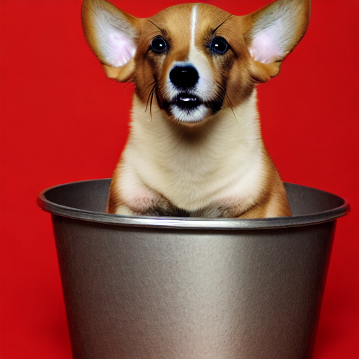
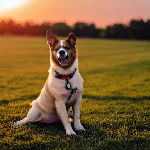
Generated Samples

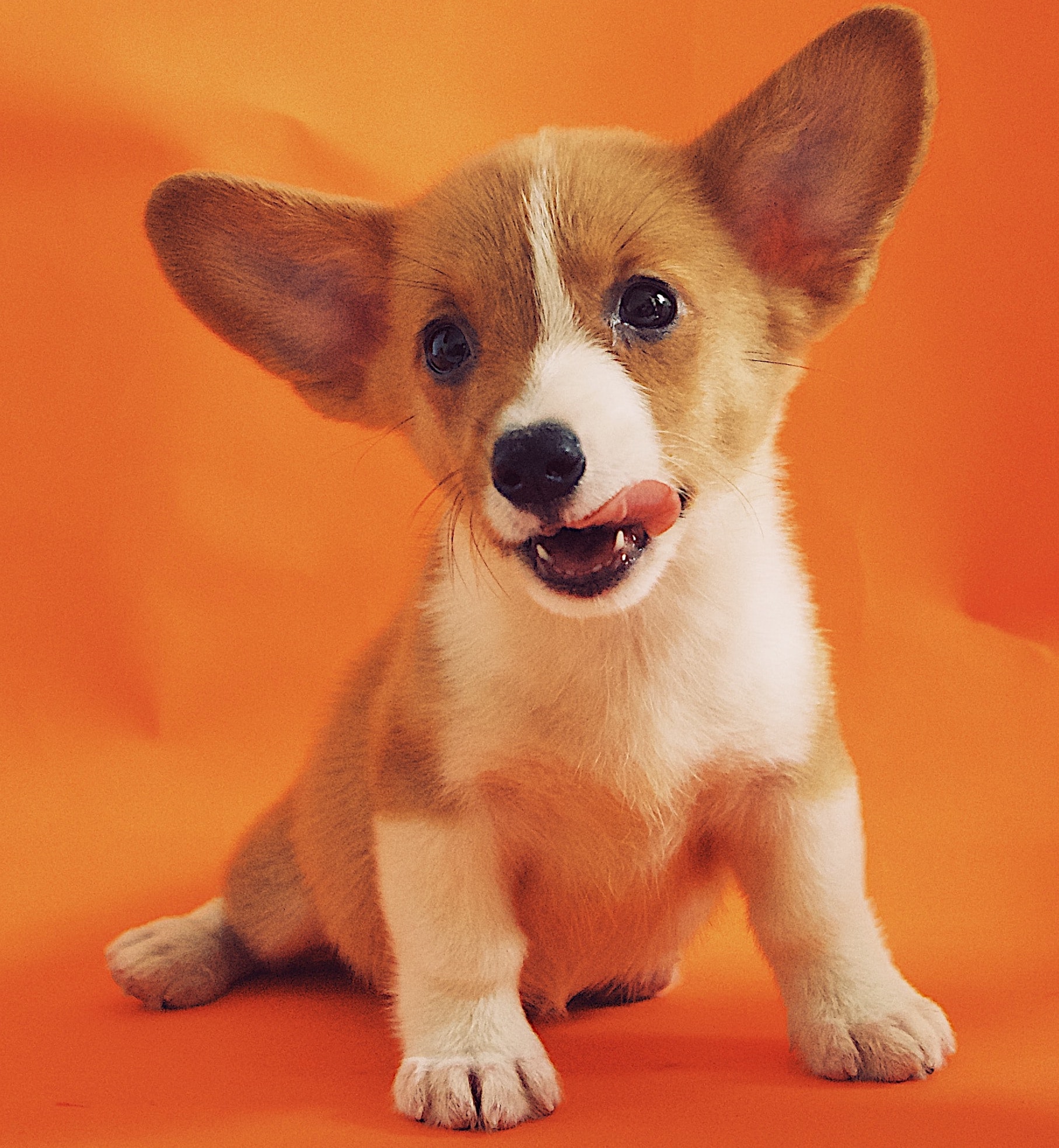
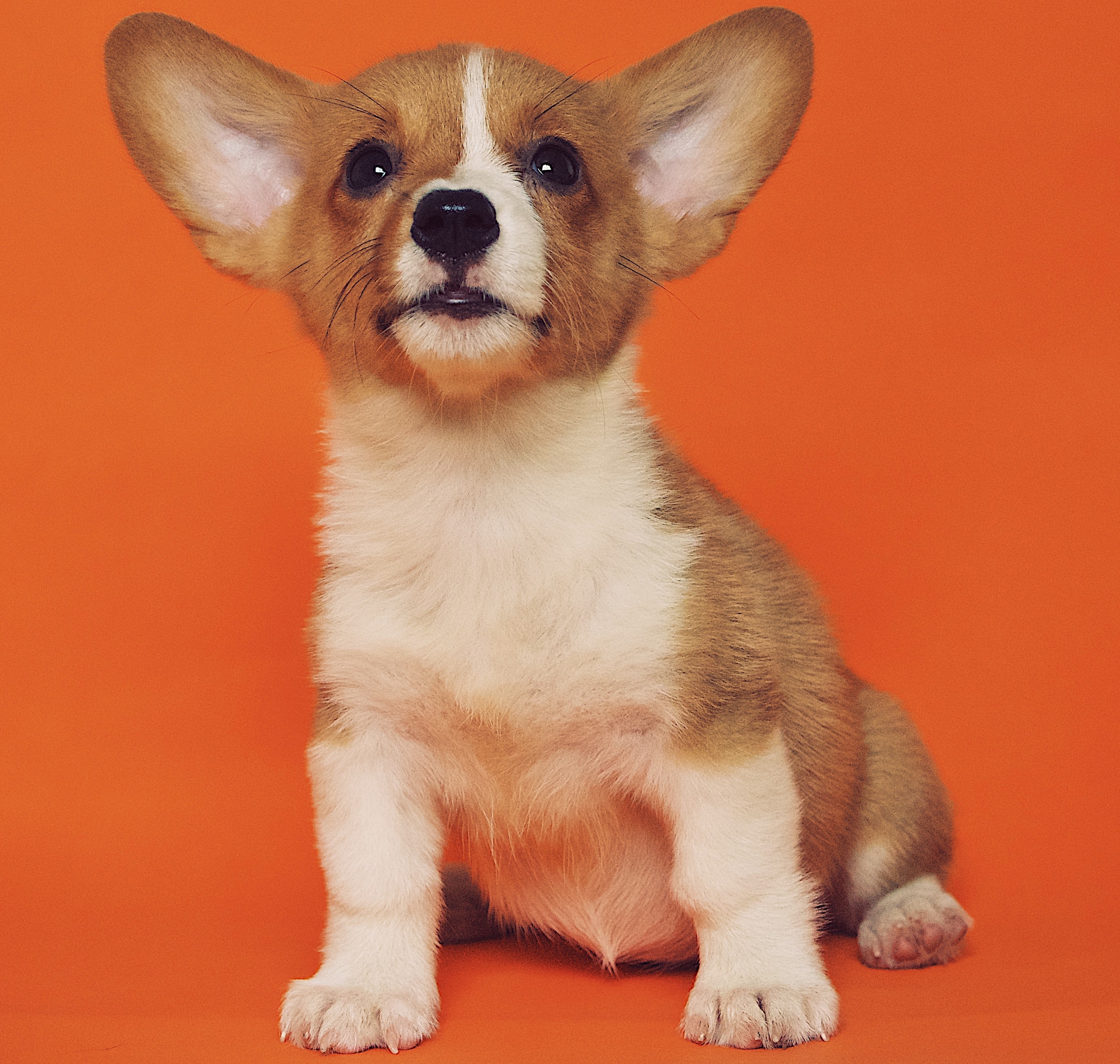
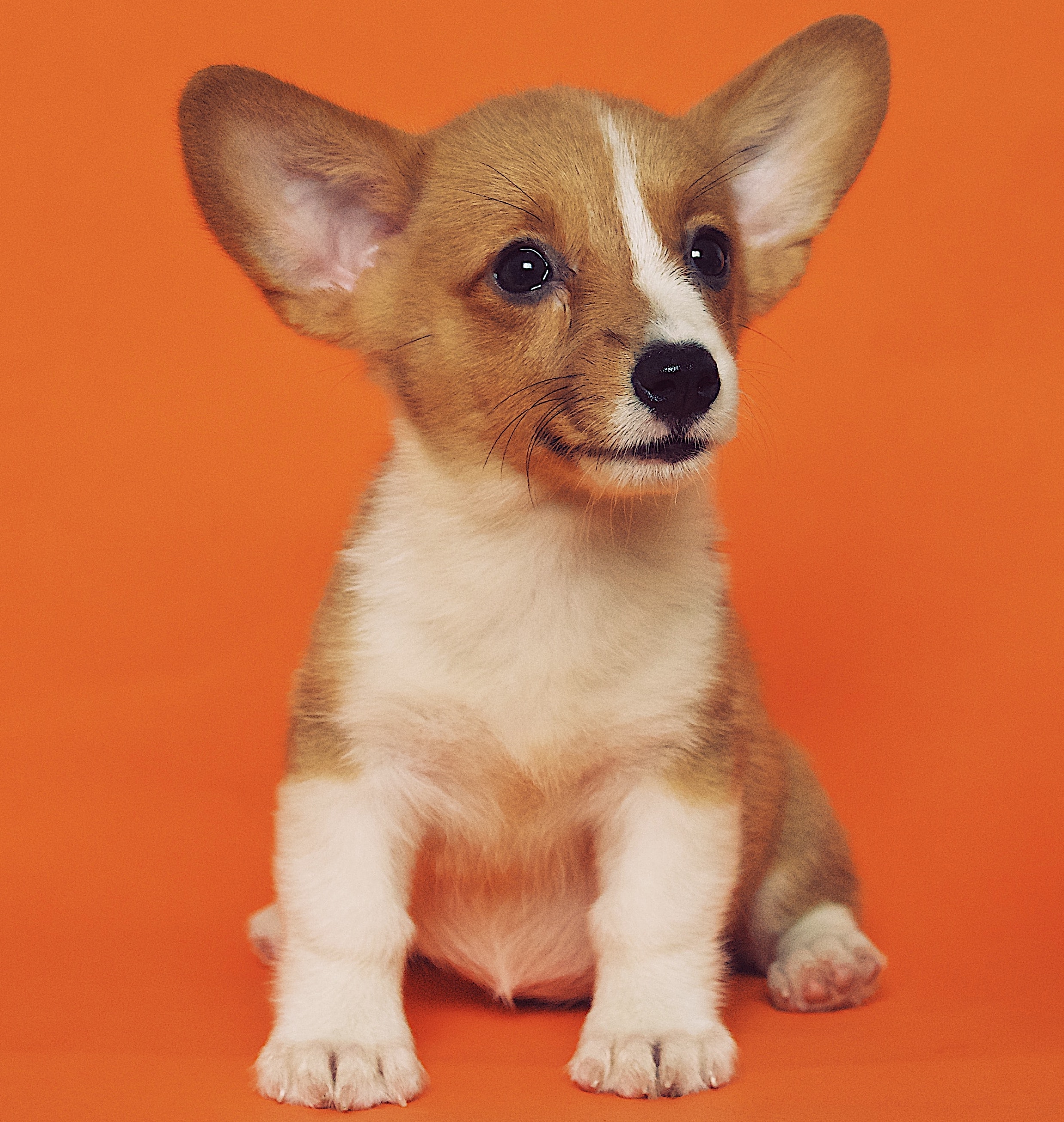
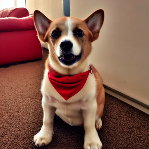
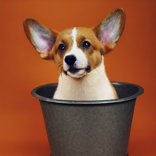
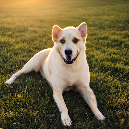
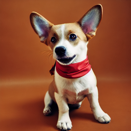
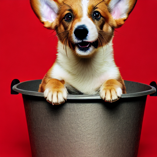
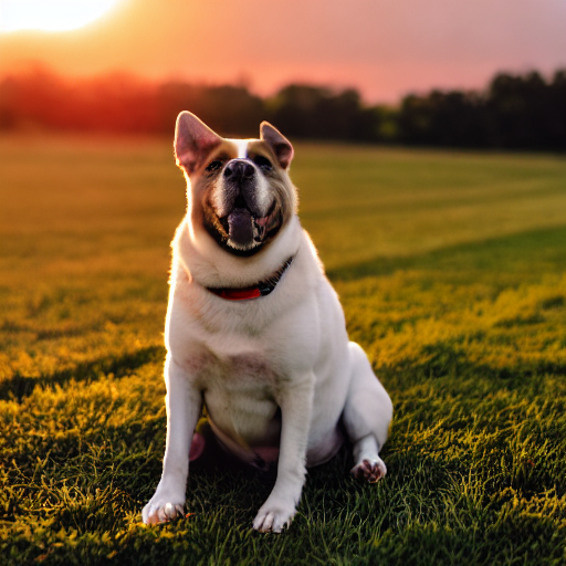
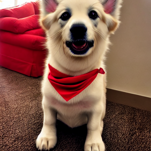
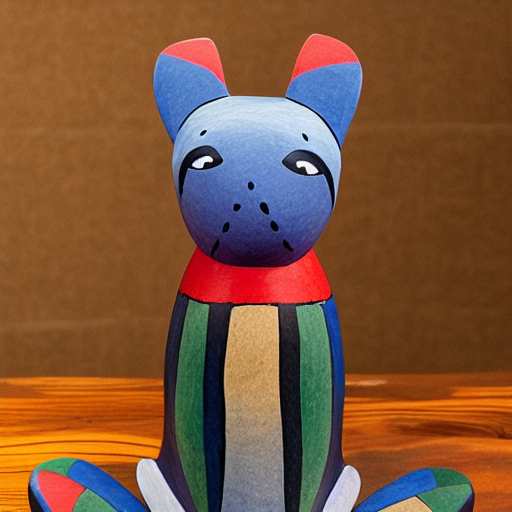
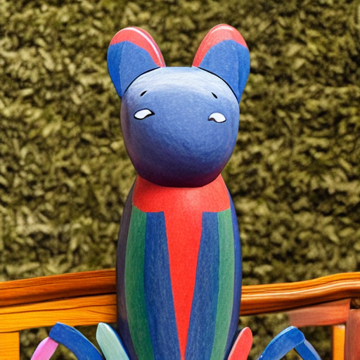
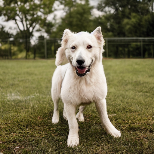
Prompts: "sks dog in a bucket" | "sks dog on grassy field" | "sks dog wearing bandana"

λ = 0.25 (best CLIP-T & DINO-I)

bucket

field

bandana

λ = 0.75 (best CLIP-I)

bucket

field

bandana

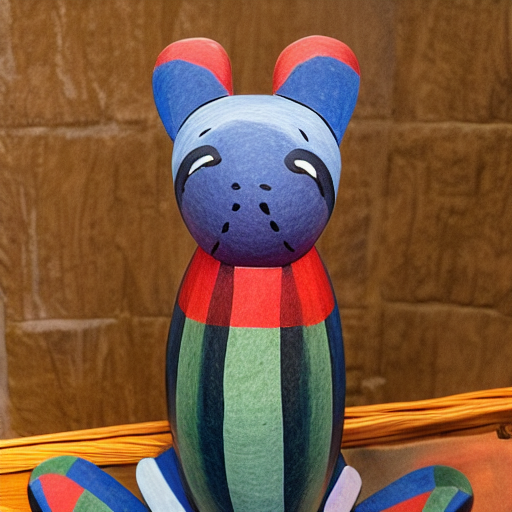
λ = 1.00 (over-regularized)

bucket

field

bandana

Key Finding: Lower λ (0.25) yields the highest CLIP-T (0.274) and DINO-I (0.588), letting the model capture subject-specific structural details. λ = 0.75 maximizes CLIP-I (0.845), preserving pixel-level visual characteristics. λ = 1.0 causes over-regularization with DINO-I dropping to 0.462. The sweet spot is λ ∈ [0.50, 0.75].

LoRA: Effect of Rank

Prompt	Rank 4	Rank 8	Rank 16
Bill Gates with a hoodie	0.242	0.172	0.172
John Oliver Naruto style	0.287	0.290	0.155
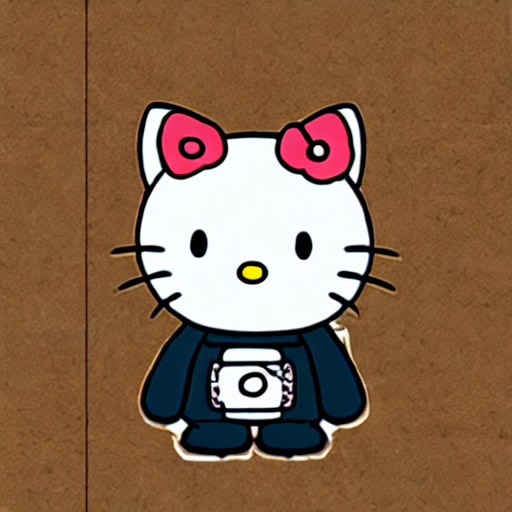
Hello Kitty Naruto style	0.314	0.277	0.253
Mickael Jackson as ninja	0.154	0.238	0.154
Mean CLIP-T	0.249	0.244	0.183

Generated Samples

Rank 4 (best overall)

Bill Gates

John Oliver

Hello Kitty

Rank 8

John Oliver

Hello Kitty

M. Jackson

Rank 16 (mode collapse)

John Oliver (collapsed)

Hello Kitty

M. Jackson (collapsed)

Key Finding: Rank 4 achieves the highest mean CLIP-T (0.249) with only ~1.6M trainable parameters. Rank 8 performs comparably (0.244) and outperforms on some prompts, suggesting prompt-dependent optimal capacity. Rank 16 suffers mode collapse, producing black/collapsed outputs (mean CLIP-T drops to 0.183). Rank 4–8 is optimal; increasing rank beyond the effective dimensionality of the style manifold is counterproductive.

Textual Inversion: Effect of Number of Vectors

Vectors	CLIP-T ↑	CLIP-I ↑	DINO-I ↑
1	0.241	0.798	0.628
2	0.237	0.819	0.664
4	0.271	0.857	0.687
8	0.277	0.834	0.690

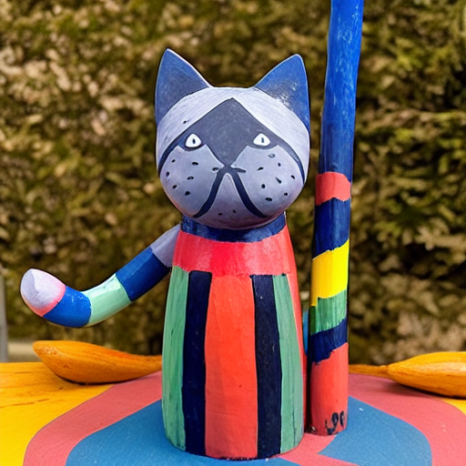
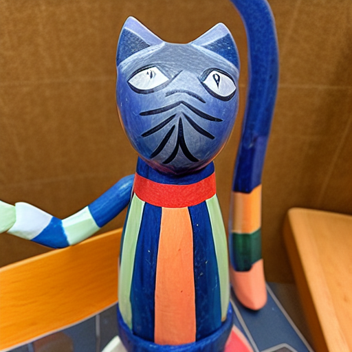
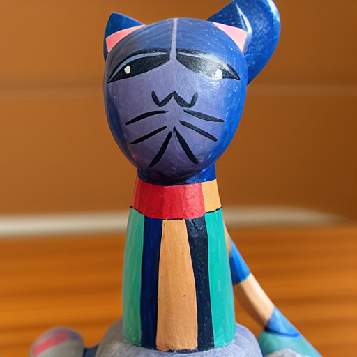
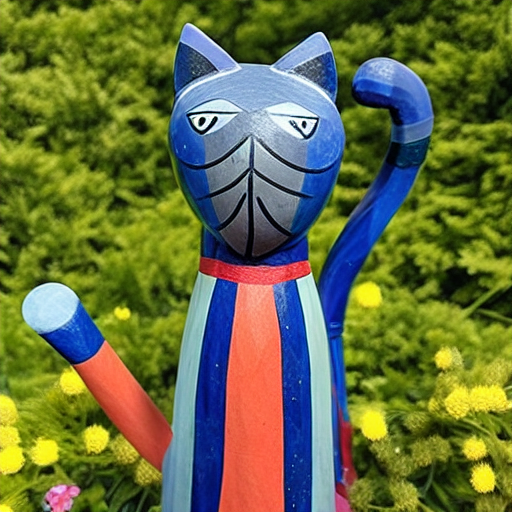
Generated Samples

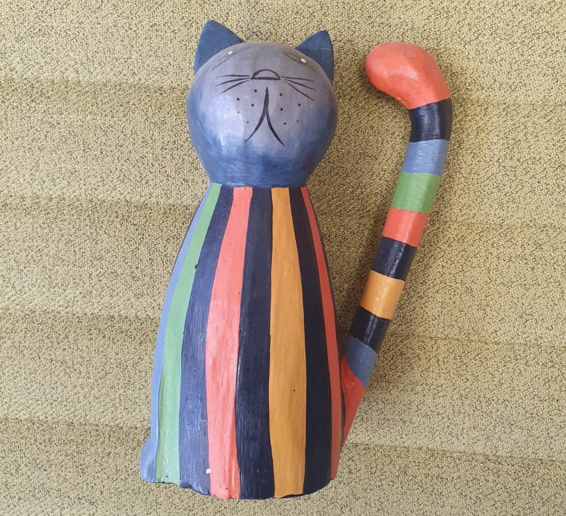
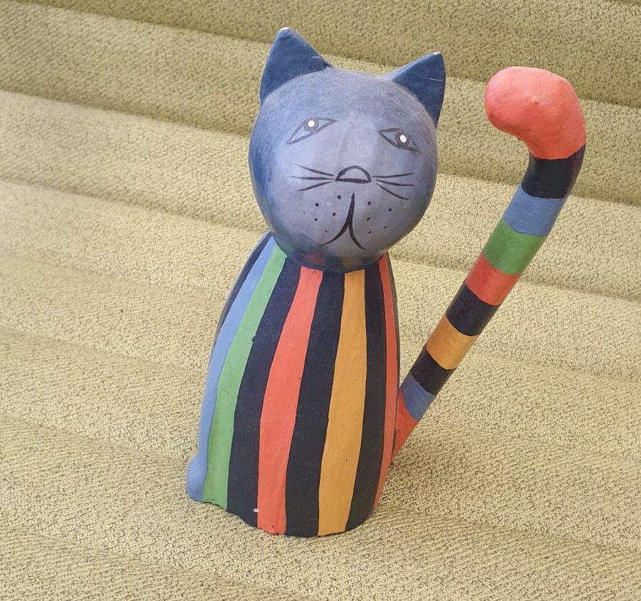
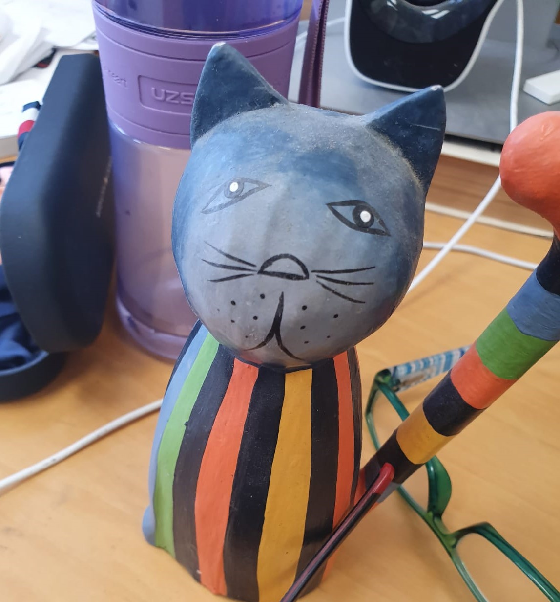
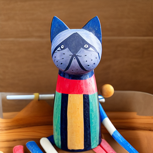
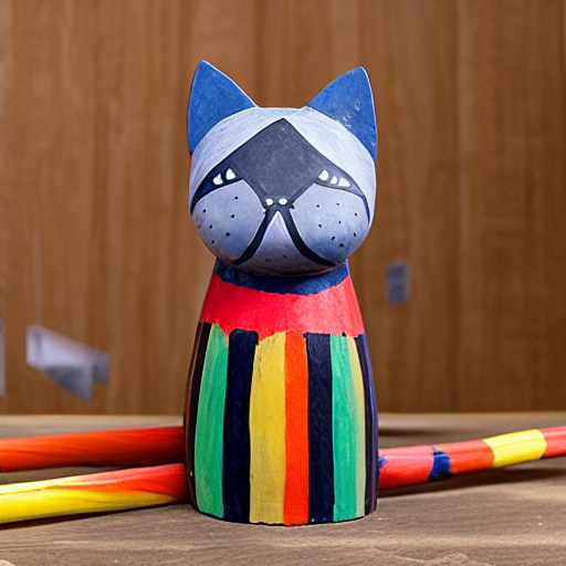
Prompts: "<sks-cat> in a basket" | "on a table" | "in a garden"

1 Vector (768 params, ~3 KB)

basket

table

garden

4 Vectors (3,072 params, ~12 KB) — best CLIP-I

basket

table

garden

8 Vectors (6,144 params, ~24 KB) — best CLIP-T & DINO-I

basket

table

garden

Key Finding: 1 vector (768 params) has insufficient capacity, yielding the lowest scores. 4 vectors peaks on CLIP-I (0.857); 8 vectors peaks on CLIP-T (0.277) and DINO-I (0.690). Remarkably, with only ~3–24 KB of storage, Textual Inversion achieves competitive or superior CLIP-I and DINO-I compared to DreamBooth's ~3.4 GB — the frozen model acts as a powerful regularizer.

Custom Diffusion Results

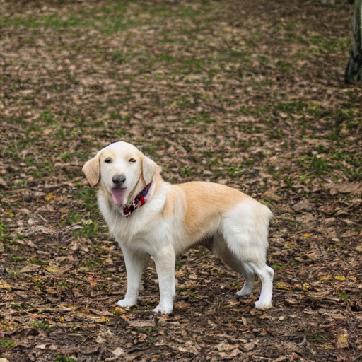
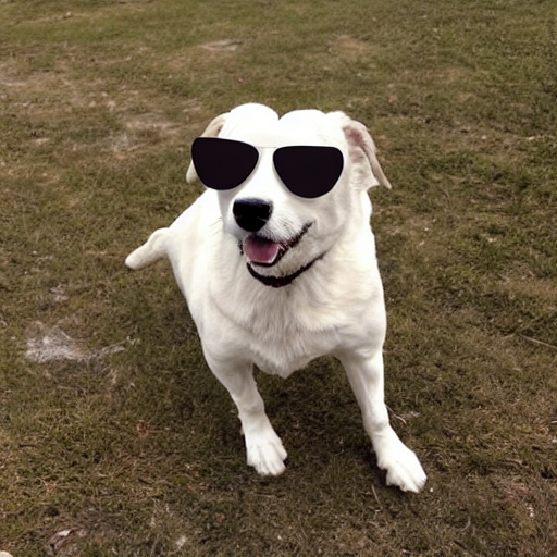
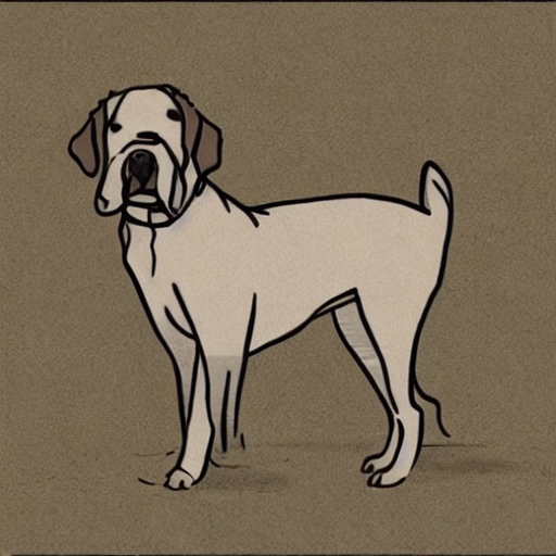
I compare two Custom Diffusion variants: crossattn (trains all cross-attention projections) vs. crossattn_kv (trains only K and V projections + modifier token). Both use 5 dog images, 250 training steps, SD v1.4, modifier token <new1>.

Variant	CLIP-T	CLIP-I	DINO-I	Latency (ms)
crossattn (all)	0.258	0.723	0.005	645
crossattn_kv	0.257	0.741	0.081	644

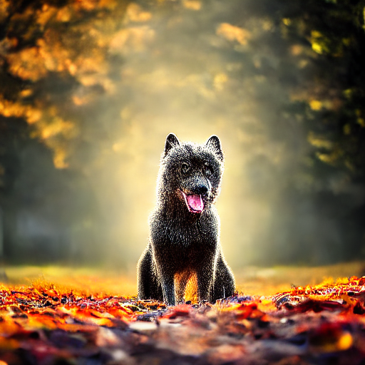
crossattn_kv (K, V only) — Best variant

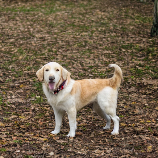
<new1> dog in the park

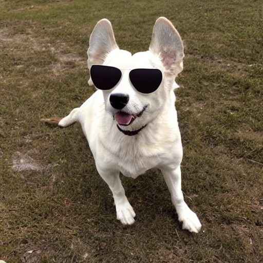
<new1> dog wearing sunglasses

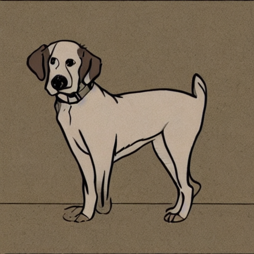
<new1> dog as a cartoon

crossattn (all cross-attention)

<new1> dog in the park

<new1> dog wearing sunglasses

<new1> dog as a cartoon

Key Finding: The crossattn_kv variant (fewer params) outperforms full crossattn on both CLIP-I (0.741 vs 0.723) and DINO-I (0.081 vs 0.005). Training additional projections introduces noise at 250 steps. The low DINO-I overall suggests more training steps would improve structural fidelity.

LCM Distillation Results

LCM targets inference speed, not subject fidelity. I compare two distillation loss variants — L2 and Huber (c=0.001) — both trained for 10k steps on LAION-CC12M from SD v1.5, generating images in only 4 denoising steps vs. 30 for other methods.

Prompt	L2 CLIP-T	Huber CLIP-T	L2 (ms)	Huber (ms)
a cat sitting on a sofa	0.280	0.266	576*	17,063*
a car parked on a street	0.191	0.247	108	111
a bowl of fruit on a table	0.293	0.257	106	107
a person riding a bicycle	0.243	0.232	106	107
Mean	0.252	0.250	224	4,347
Mean (excl. warmup)	—	—	108	108

* First image includes GPU warmup overhead (varies across runs). Steady-state latency is identical for both loss variants.

Latency Comparison Across Methods

Method	Inference Steps	Latency (ms)	Speedup
DreamBooth (λ=0.75)	30	2,913	1.0×
LoRA (r=8)	30	835	3.5×
Custom Diff. (kv)	30	644	4.5×
Textual Inv. (4 vec)	30	613	4.8×
LCM (L2 / Huber)	4	108	27.0×

LCM Generated Samples — L2 Loss (4 steps)

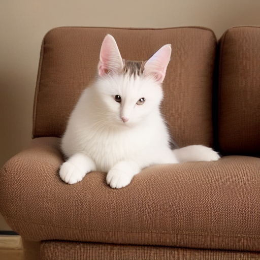
cat on sofa

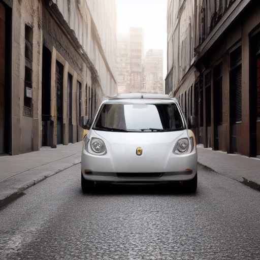
car on street

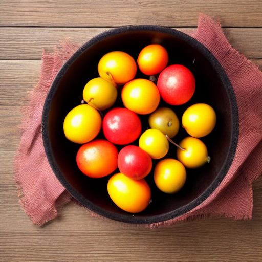
fruit bowl

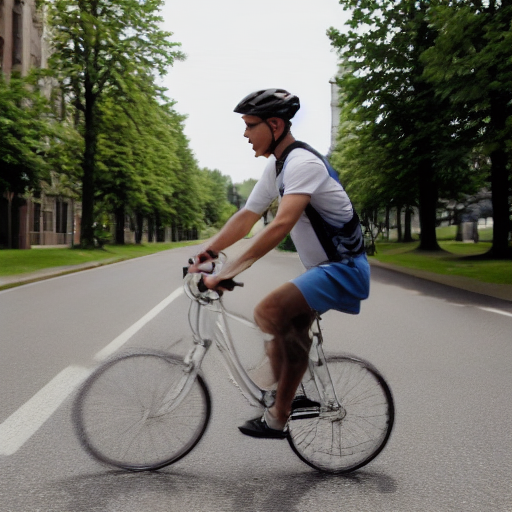
person on bicycle

LCM Generated Samples — Huber Loss (4 steps)

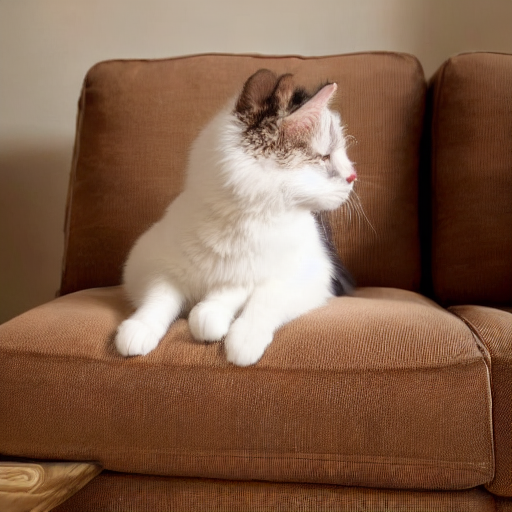
cat on sofa

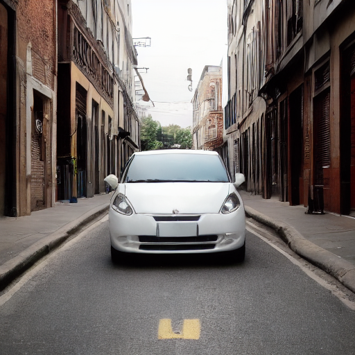
car on street

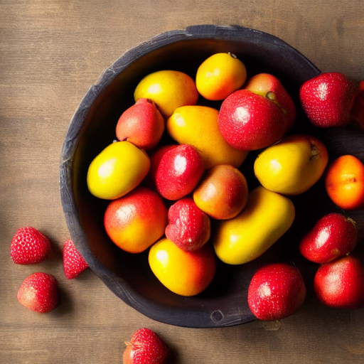
fruit bowl

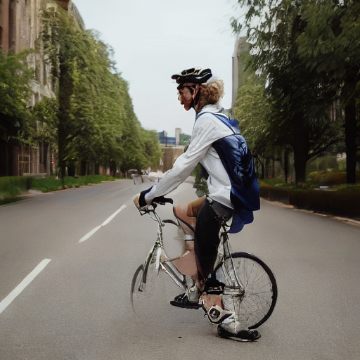
person on bicycle

Key Finding: Both L2 and Huber loss variants achieve identical steady-state latency (~108ms), a ~27× speedup over standard 30-step inference (2,913ms). CLIP-T scores are comparable (L2: 0.252, Huber: 0.250), confirming that the loss function affects neither speed nor text-image alignment. L2 shows higher per-prompt variance (0.191–0.293 vs. 0.232–0.266 for Huber).

DDPO Results

DDPO uses reinforcement learning with an aesthetic reward function. I compare two variants: No LoRA (full U-Net RL fine-tuning) and LoRA (RL fine-tuning with low-rank adapters), both trained for 200 epochs on SD v1.5, evaluated with 50 inference steps at guidance 7.5.

Prompt	Aesthetic Score		CLIP-T		Latency (ms)
	No-LoRA	LoRA	No-LoRA	LoRA	No-LoRA	LoRA
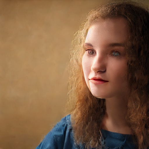
portrait (soft lighting)	6.14	5.67	0.208	0.217	3,629*	16,589*
landscape (mountains)	6.32	6.57	0.252	0.251	1,216	1,190
dog in a park	5.12	6.78	0.205	0.204	1,199	1,190
futuristic city (neon)	6.61	6.09	0.260	0.258	1,202	1,181
Mean	6.05	6.28	0.231	0.232	1,812	5,038
Mean (excl. warmup)	—	—	—	—	1,206	1,187

* First image includes GPU warmup overhead (varies across runs).

DDPO Generated Samples — No-LoRA (full U-Net RL)

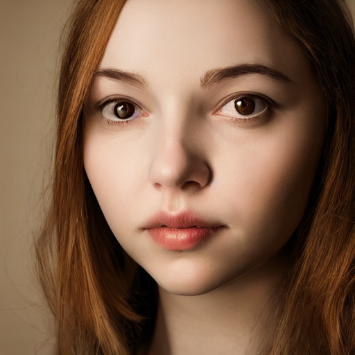
portrait

landscape

dog in park

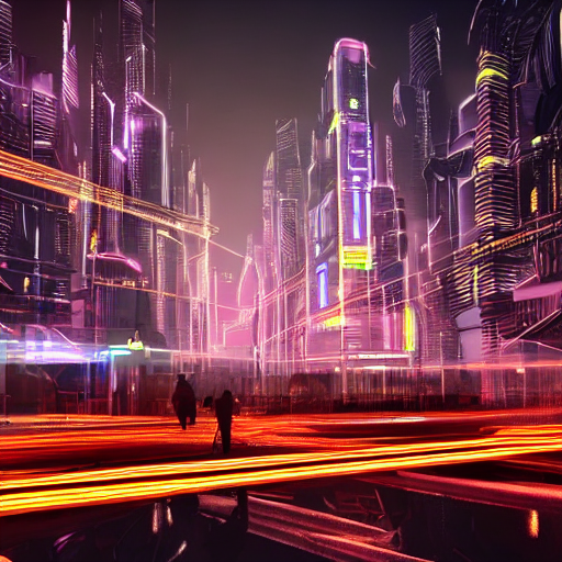
city neon

DDPO Generated Samples — LoRA

portrait

landscape

dog in park

city neon

Key Finding: The LoRA variant achieves a higher mean aesthetic score (6.28 vs. 6.05) despite training fewer parameters, suggesting LoRA's constrained parameter space regularizes reward optimization. Both variants produce comparable CLIP-T (~0.23) and steady-state latency (~1,190ms). The "dog in a park" prompt shows the largest LoRA improvement (6.78 vs. 5.12).

Property	DreamBooth	LoRA	Textual Inv.	Custom Diff.	LCM	DDPO
What's trained	Entire U-Net	Low-rank adapters	Embedding only	Cross-attn K,V + token	Student model	U-Net (RL)
Trainable params	~860M	~1.6-6.4M	~768-6,144	~57M (~2%)	Full model	Full model
Storage	~3.4 GB	~3 MB	~3-24 KB	~75 MB	~3.4 GB	~3.4 GB
Best CLIP-T	0.274	0.249	0.277	0.258	0.252	0.232
Best CLIP-I	0.845	N/A	0.857	0.741	N/A*	N/A*
Best DINO-I	0.588	N/A	0.690	0.081	N/A*	N/A*
Aesthetic	—	—	—	—	—	6.28
Latency	2,913ms	835ms	613ms	644ms	108ms	1,187ms
Inference	Normal	Normal (merged)	Normal	Normal	~27× faster	Normal (50 steps)
Multi-concept	No	Additive	No	Native	No	No

The Personalization Problem

Five Approaches, One Goal

DreamBooth

LoRA

Textual Inversion

LCM Distillation

Custom Diffusion

DDPO

Evaluation Metrics — How Do I Measure Success?

CLIP-T — Text-Image Alignment

Why is this important?

CLIP-I — Image-Image Similarity

Why is this important?

DINO-I — Structural / Identity Similarity

Why is this important?

How Each Method Works

DreamBooth — Fine-Tuning the Entire Model

Architecture Deep Dive: What Happens During Training

Why does prior preservation matter?

LoRA — Low-Rank Adaptation

Architecture Deep Dive: Low-Rank Decomposition in Attention

What does rank r actually control?

Textual Inversion — Teaching Through Words

Architecture Deep Dive: How a Single Embedding Captures a Concept

Why does this work at all with so few parameters?

Latent Consistency Distillation

Architecture Deep Dive: From Multi-Step ODE to One-Step Prediction

Custom Diffusion — Selective Cross-Attention Fine-Tuning

Architecture Deep Dive: Why Cross-Attention K & V Are the Sweet Spot

Why are K and V projections so special?

DDPO — Reinforcement Learning Meets Diffusion

Architecture Deep Dive: Denoising as a Markov Decision Process

Why is RL-based optimization game-changing for personalization?

Architecture Animations

Experimental Setup

Input Datasets

Dog — DreamBooth (3 imgs) & Custom Diffusion (5 imgs)

Cat toy — Textual Inversion (3 images)

Large-scale Datasets

Results

DreamBooth: Effect of Prior Weight λ

Generated Samples

LoRA: Effect of Rank

Generated Samples

Textual Inversion: Effect of Number of Vectors

Generated Samples

Custom Diffusion Results

crossattn_kv (K, V only) — Best variant

crossattn (all cross-attention)

LCM Distillation Results

Latency Comparison Across Methods

LCM Generated Samples — L2 Loss (4 steps)

LCM Generated Samples — Huber Loss (4 steps)

DDPO Results

DDPO Generated Samples — No-LoRA (full U-Net RL)

DDPO Generated Samples — LoRA

Method Comparison

The Fidelity–Efficiency Spectrum